Geospatial Data Sources
Today, an abundance of open data are available for geospatial analysis. In the Open Data Handbook, open data are defined as follows:
Open data is data that can be freely used, re-used and redistributed by anyone - subject only, at most, to the requirement to attribute and sharealike.
This document provides some background and insight on open data sources used for geospatial analysis after a brief review of geospatial data structures and important concepts to consider when working with geospatial data.
This notebook is organized as follows:
What is geospatial data?
Spatial Data
Introductory courses on Geographic Information Systems (GIS) typically differentiate between spatial data and attribute data.
Spatial datasets contain data about geographic entities or features defined using coordinate and projection information that reference locations on Earth.
Geographic entities or features are digitally represented using vector geometry or raster (grid) structures.
Vector Data
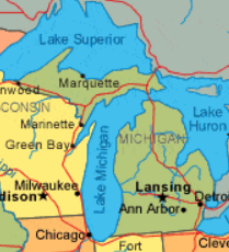
Basic vector structures include points, lines, and polygons. These objects may be grouped as collections (multi-points, multi-lines, and multi-polygons) to avoid data redundancy. For example, the state of Michigan is digitally represented with two polygons (the glove and the Upper Pennisula) separated by Lake Michigan. However, these two polygons are stored in open datasets as a multi-polygon because they both represent the same geographic entity, the state of Michigan.
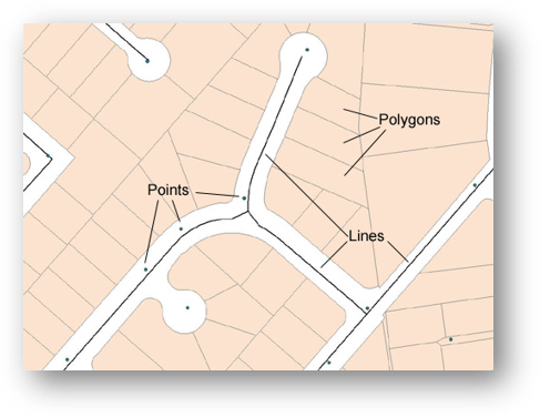
Points are stored using a single coordinate pair (x,y) or (y,x) where often x = longitude and y = latitude (unprojected geographic coordinates).
Lines or polylines are defined using at least two different coordinates, with additional coordinates providing shape to the line (x1,y1) ...(xn,yn).
Polygons are polylines where the first and last coordinate are the same. In other words, a polygon is a closed polyline.
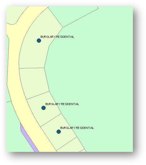
POINTS
- Represent discrete locations
- a single coordinate pair (x,y)
- often x = longitude and y = latitude (unprojected geographic coordinates).
EXAMPLES
- Physical entities
- Trees
- Police Camera Locations
- ATM machines
- Bus Stops
- Events
- Crimes
- Towed vehicle location
- Parking citation location
Back to TOP
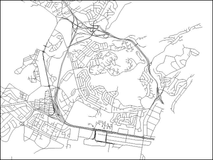
LINES or POLYLINES
- at least two different coordinate pairs
- with additional coordinates providing shape to the line (x1,y1) ...(xn,yn).
- typically represent the centerline of a feature
EXAMPLES
- Physical entities
- streets
- rivers
- hiking trails
- Events
- bus routes
- race routes
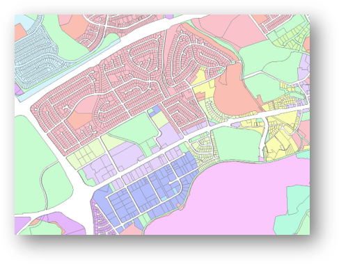
POLYGONS
- polylines where the first and last coordinate pairs are the same.
- a polygon is a closed polyline
- many polygons in GIS represent boundaries that cannot be seen and are subject to change
EXAMPLES
- Physical entities
- building footprint
- lake
- Events
- parcel boundary
- police district
- census tract
- school district
- county boundary
Back to TOP
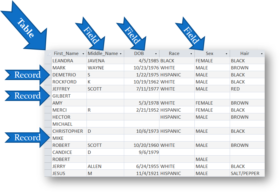
TABLES
- Vector data typically are represented in tables.
- Tables contain records or rows of horizontal data
- Generally, in spatial datasets one row (record) in a table represents one geographic entity or event
- Most tables contain a "header row" that identifies the information in each column
- Records are composed of fields (columns of vertical data)
- Spatial datasets contain at least one field with geometry data (the shape field in an ArcGIS dataset)
- A table may contain spatial data (coordinate information) and geographic identifiers
- A table may contain additional attributes (characteristics) for each geographic entity
Example, a spatial database of U. S. states would contain 50 rows (+ a header row) each with coordinates for polygons or multi-polygons and the state name or FIPS code.
One record per entity is NOT a database rule, however, so the user should check the data before using it. One clue is repeated spatial (GEO or OBJECT) IDs for records. Other datasets can have multiple records for the same location. For example, a dataset on crimes or vehicle crashes may have more than one event at a specific location.
Some tables may contain only attribute information with a geographic identifier that may be used to join the attributes to spatial data. For example, census tables contain GEOIDs that identify the geographic entity that the data describes. So data for census tracts (like population, median income, ...) can be joined to a census tract spatial dataset for mapping and analysis.
Common formats for storing vector data are GeoJSON, .shp (ESRI shapefile), and WKT (well-known text). For more information see GeoJSON data format.
Back to TOP
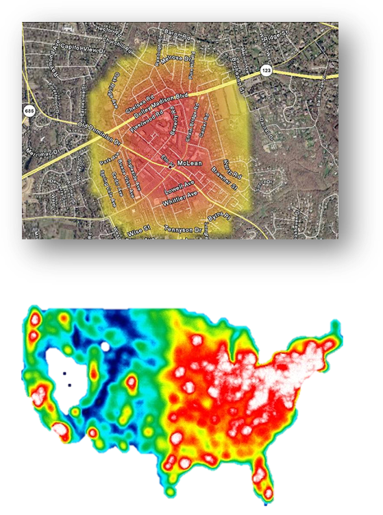
RASTERS
- Raster data structures typically are same sized rectangular (grid) cells.
- Resolution indicates the amount of earth covered by a cell.
- For instance, a raster data set with 500 meter resolution means that each cell represents 500 by 500 meters on the earth.
- Raster data structures are used to represent geographic entities that are continuous over space, like elevation.
- Whereas vector data structures are used to represent man-made entities (like roads and buildings) or features with well defined boundaries (like states and counties).
Examples of raster data include:
- Precipitation
- Elevation (or depth)
- Temperature
- Crime hot spots (derived from point data)
Back to TOP
Important Spatial Data Concepts
Every geographic entity or event in a spatial dataset has a unique ID. Always check to see if there are duplicate IDs in a data table. If there are, find out why!
The example shared in class was a Kaggle dateset on restaurants produced from a search for Vegan Restaurants. The table contained 10,000 records but each record DID NOT represent a different restaurant. Each record represented a MENU ITEM at a restaurant, so there were many records for each restaurant and each individual restaurant had unique point coordinates. The dataset contained information for just over 200 restaurants, not 10,000, so it was a sample of U.S. restaurants.
The situation described above is different from that of a dataset with all unique IDs but non-unique locations. For example, crime datasets have unique IDs for each crime event but if multiple crimes occur at the same address, the point locations are the same. When visualizing this data we can use graduated symbol sizes to represent the number of events at a particular location.
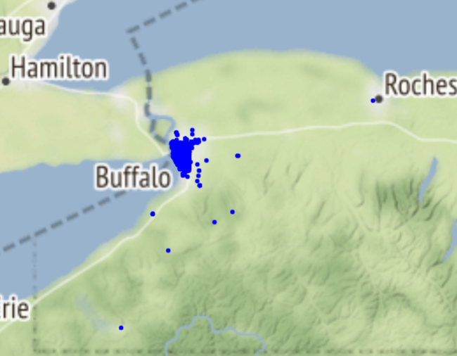
Often it is necessry to check the positional validity of points in a dataset. For example, a crime dataset from the Buffalo Police Department should contain point locations of crimes in Buffalo, NY. The Buffalo police do not respond to calls in surrounding towns. The city boundary is needed to determine if all of the points fall within the city. Analysts should make sure locations in a dataset make sense given what the dataset represents. The image below shows crime locations from the 2014 Buffalo Crime incident data. As you can see, there are many locations outside of the city.
Another common problem with open datasets (point data) is missing location information. There may be a record for an event but no coordinate. Analysts must decide if proper conclusions can be drawn regardless of the missing locations. In general, if over 10% of the point locations are missing, the data is unreliable for spatial analysis. There are methods to interpolate missing locations but these rely on other information about the event.
Polylines typically represent the centerline of a geographic entity (like a river or road). Some roads (particularly divided highways) are represented as two polylines, one for each direction of travel. Typically, width is an attribute of the centerline that may be used to offset geocoded addresses or expand a buffer or search tolerance.
Some databases represent a linear feature by its two edges, like each bank of a river. Since these edges belong to the same geographic entity, they are often stored as multi-polylines. Other polyline entities may represent the actual location of an entity (utility line, pipeline, curb).
Most linear features are composed of many smaller segments. For example, roads may be composed of many segments representing intersections with other roads, boundaries, and/or utility lines. Depending on the type of analysis, it may be beneficial to merge these segments into a single feature, like a bus route.
The mathematical set theory concept "mutually exclusive and collectively exhaustive" is pertinent to polygon data. Polygons (and raster cells) may be space-filling (collectively exhaustive), meaning every location in the study area is "assigned to" a polygon. In other words, there are no holes.
An example of space filling vector geographies is the Census Hierarchy. Every location in the U.S. is assigned to a block, block group, tract, ...., State, Region, Division.
Examples of non-space filling polygon geography are census designated places (cities, towns, villages, etc.), urban areas, and metro and micropolitan statistical areas. Every location in the U.S. is not assigned to a place.
Polygon layers that are "mutually exclusive" have no area of intersection or overlap. An example is county boundaries; no two counties overlap. Alternatively, buffer polygons around several geographic entities may overlap, such as buffers representing the market area for grocery stores or noise levels near highways.
Non-overlapping geographies allow for nested IDs to facilitate analysis. Since a census tract falls entirely within a county and each tract is in one and only one county, the tract ID contains the State FIPS, County FIPS and tract. Only a single layer of tract boundaries is required to identify all tracts in Erie County, NY, namely tract ids that begin with '36029'. Zip codes can cross county boundaries, so each zip code has a 5 (or nine) digit unique ID. Thus, to find all zip codes in Erie County, NY, two feature layers are required, one with zip code boundaries and the other with county boundaries. Part of some zip codes will fall into adjacent counties, making summarizing zip code data by county more challenging.
Back to TOP
Important Spatial Data Concepts
ATTRIBUTE DATA
Attribute data are data that describe characteristics of geographic entities. For example, in a tree inventory, the spatial data will be points (coordinate pairs). For each point (tree), there is attribute information that describes trees, like species, height, crown circumference, etc. Attributes are stored in columns of a digital table. Each column (aka field) is defined by digital data types (i.e. text/string, number, boolean...). Typically, the data type of each attribute field is part of the metadata for an open dataset.
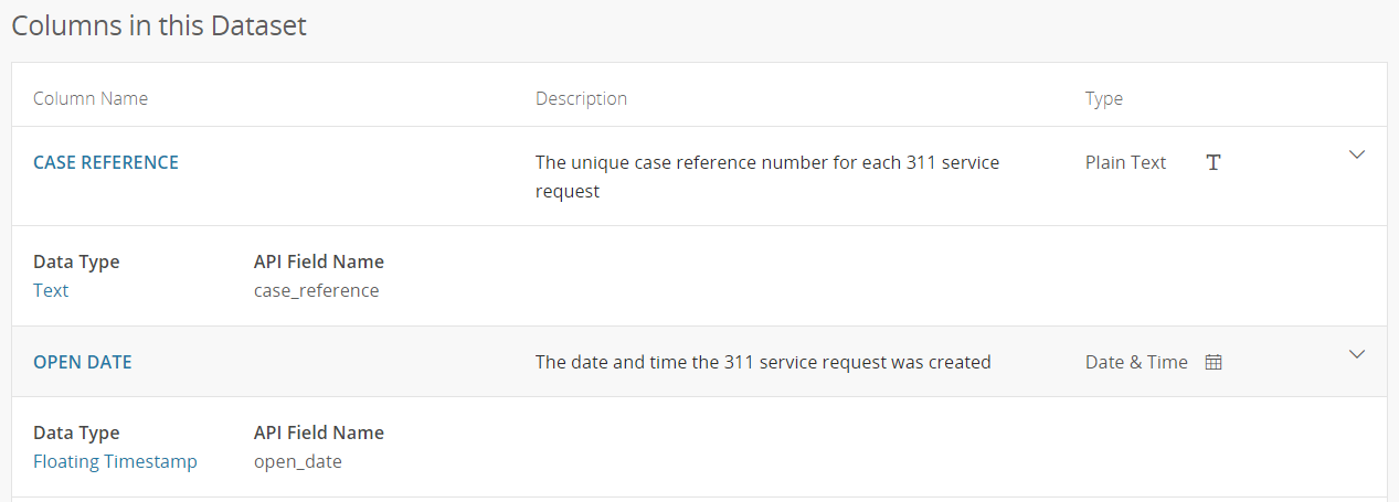
One of the most common issues with attribute data is missing data. Analysts must decide how missing data might impact the results of the analysis.
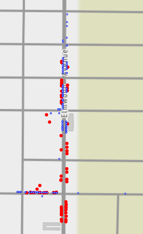
Another common problem with attribute data is inconsistencies. The image below shows meter locations (red dots) and parking violations along a section of Elmwood Avenue in Buffalo, NY. Both datasets were accessed on the Buffalo Open data site. The parking violations are "Meter Overtime" only. There are several violations at locations where meters do not exist and there are several meters with no violations.
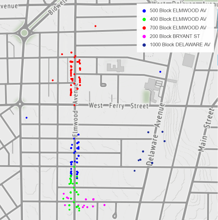
Another example is from a crime incident dataset that contains a descriptive location of where a crime occured along with the actual coordinates. Notice that the 500 and 700 blocks of Elmwood include point locations not along Elmwood. There are points described as the 400 block of Elmwood mixed in with locations described as the 500 block of Elmwood and vice versa. This is only a small subset of the data.
THE FIRST JOB FOR AN ANALYST IS TO UNDERSTAND THE DATA!
Back to TOP
Open Data
There are hundreds, if not thousands, of open data portals. Links to some are provided below.
- Open government: Data.gov
- European Union Open Data Portal
- New York State Open Data
- New York City Open Data
- City of Buffalo, NY Open Data
- Forbes story: links to 50+ state open data portals
- Forbes story: links to 85 municipal open data portals
The next notebook covers basic information about reading geospatial data from open data sets.